ELBO Surgery
tldr: The ubiquitous isotropic Gaussian prior for generative models doesn't make sense / doesn't work, which motivates work on priors.
At NIPS, Dawen Liang mentioned Hoffman & Johnson's ELBO surgery paper offhand while talking about tuning KL divergences, and it's very interesting, so I thought I'd go over it. It's very clearly written, so I won't go into any of the derivations, but instead offer my interpretation.
Motivation
I worked in the past on applying variational inference and comparing it to models trained via MAP/MLE inference. I decomposed the evidence lower bound (ELBO) as:
This is, I think, the most common interpretation: split the ELBO into a reconstruction term and a KL divergence term. The first encourages the model to reconstruct the data, and the second regularizes the model, asking the posterior distribution over $z_n$ to have a certain shape, like a Gaussian. For example, in a VAE the second term is what prevents the model from just learning a Dirac delta-like posterior $q(z_n | x_n) \sim \mathcal{N}(x_n, 0.001)$ around the original value1.
In the NLP world, people have seen some problems though - when we have a very powerful generative model (e.g., an RNN), the KL divergence can vanish. This means the posterior $q(z_n | x_n) \approx p(z_n)$ learns nothing about the data, so the generative model $p(x_n | z_n)$ becomes like a language model. The usual trick is to anneal the KL divergence term in, so that that inference can be useful. A lot of people are unhappy with this because it adds extra hyperparameters and it feels really non-Bayesian.
Contribution
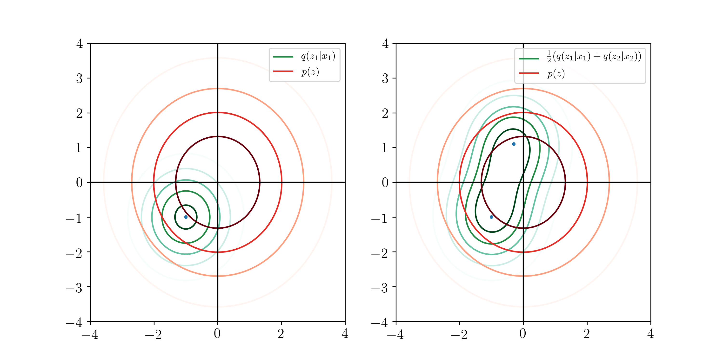
The contribution of this paper is the following observation: the KL divergence above measures the distance from the posterior for a single $z_n$ to the prior, but we really care about the KL divergence from the average posterior over all data points to the prior. So they define
which is the average posterior we see. The intuition here is that when we're trying to do inference, we shouldn't exactly be penalized for being very confident in $q(z_n | x_n)$. However, we want the average distribution to be close to the prior, so this term can go to 0 safely without worrying about whether the posterior has learned something. In fact, at the cost of a lot of extra computation, we can even safely set the prior to be this distribution, or let $p(z) \triangleq q(z)$! 

Then, they view $n$, the index variable, as a random variable, where the interpretation is that our generative model samples $n \sim \operatorname{Unif}[N]$, and then picks a $z_n$ from $p(z)$. This isn't totally intuitive, but it makes more sense on the inference side, which we'll see below. Finally, they decompose the second term further as follows:
(this is not an obvious derivation, but the math checks out). Here, $q(n | z)$ (which we can decompose using Bayes' law) can be interpreted as 'the distribution over which datapoint this $z$ belongs to'. The description 'index-code mutual information' comes from an alternative way to write the expression, but I like this one more. Also, they upper bound this value by $\log N$, a not insignificant quantity! This is 11 nats on MNIST.
Experiments
Finally, the most interesting section, which is the quantitative analysis: they apply the model to a set of the usual VAEs with an isotropic Gaussian prior used for binarized MNIST, and get the following results:
| ELBO | Average KL | Mutual info. | Marginal KL | |
|---|---|---|---|---|
| 2D latents | -129.63 | 7.41 | 7.20 | 0.21 |
| 10D latents | -88.95 | 19.17 | 10.82 | 8.35 |
| 20D latents | -87.45 | 20.2 | 10.67 | 9.53 |
So, what's going on is that as we increase the number of latent dimensions to 10/20, the marginal KL gets large! Which means that the Gaussian prior is not good enough anymore. At least, that's my interpretation. This is interesting food for thought, since that gives a lot of evidence for a hunch that people have had for a while (and motivates work on new prior distributions, like our paper).